Lecture 8
Introduction to Apache Spark
Looking Back
- Distributed File Systems (HDFS)
- Data locality and fault tolerance
- Commodity hardware clusters
- Why distributed storage matters
Today
- From HDFS to distributed computation
- Introduction to Apache Spark
- Spark RDDs
- Spark DataFrames
- SparkSQL
Why Spark? From Hadoop to In-Memory Computing
Starting with our BIG dataset
The data is split

The data is distributed across a cluster of machines
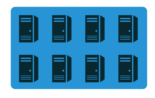
You can think of your split/distributed data as a single collection.
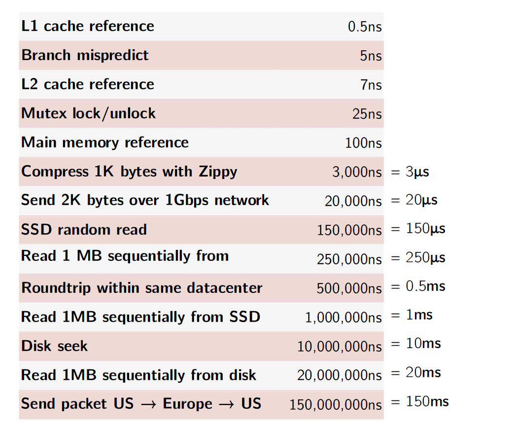
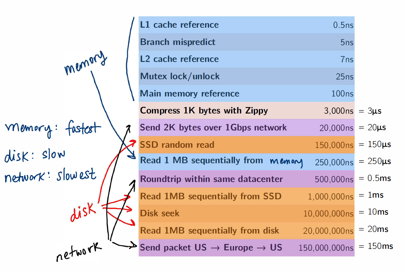
Important Latency Numbers
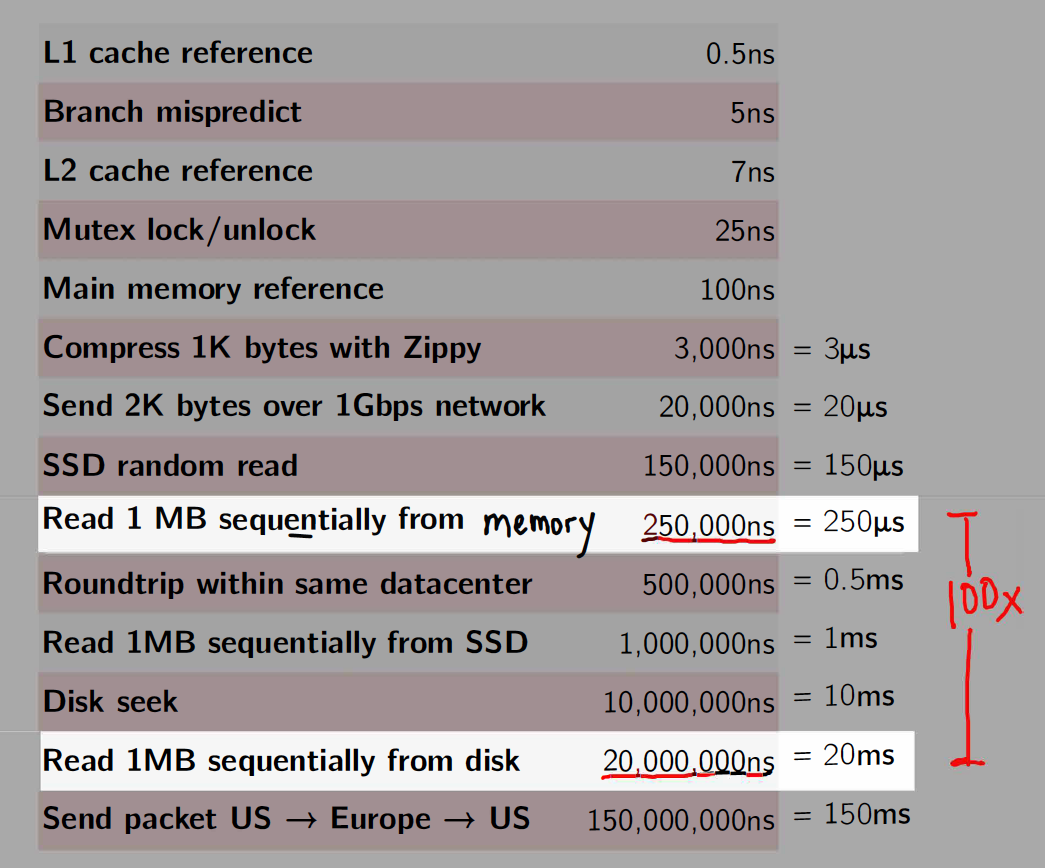
Memory vs. Disk
Memory vs. Network
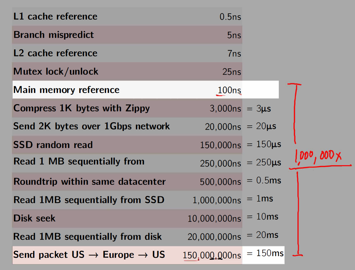
Memory, Disk and Network
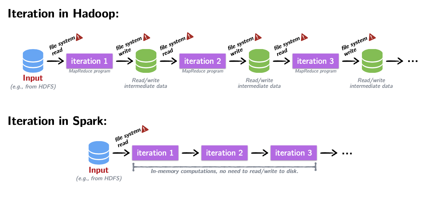
MapReduce/Hadoop was groundbreaking
It provided a simple API (map and reduce steps)
It provided fault tolerance, which made it possible to scale to 100s/1000s of nodes of commodity machines where the likelihood of a node failing midway through a job was very high
- Computations on very large datasets failed and recovered and jobs completed
Fault tolerance came at a cost!
- Between each map and reduce step, MapReduce shuffles its data and writes intermediate data to disk
- Reading/writing to disk is 100x slower than in-memory
- Network communication is 1,000,000x slower than in-memory
Introducing Spark: a Unified Engine
What is Spark
![]()
A simple programming model that can capture streaming, batch, and interactive workloads
Retains fault-tolerance
Uses a different strategy for handling latency: it keeps all data immutable and in memory
Provides speed and flexibility
Spark Stack
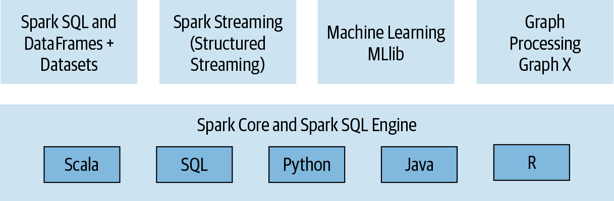
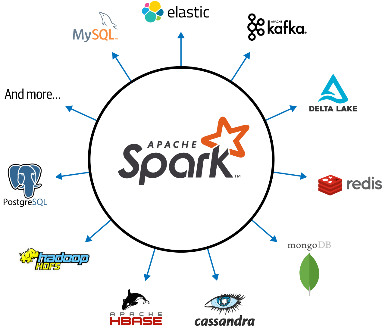
Connected and extensible
Three data structure APIs
RDDs (Resilient Distributed Datasets)
DataFrames SQL-like structured datasets with query operations
Datasets A mixture of RDDs and DataFrames
We’ll primarily use RDDs and DataFrames in this course.
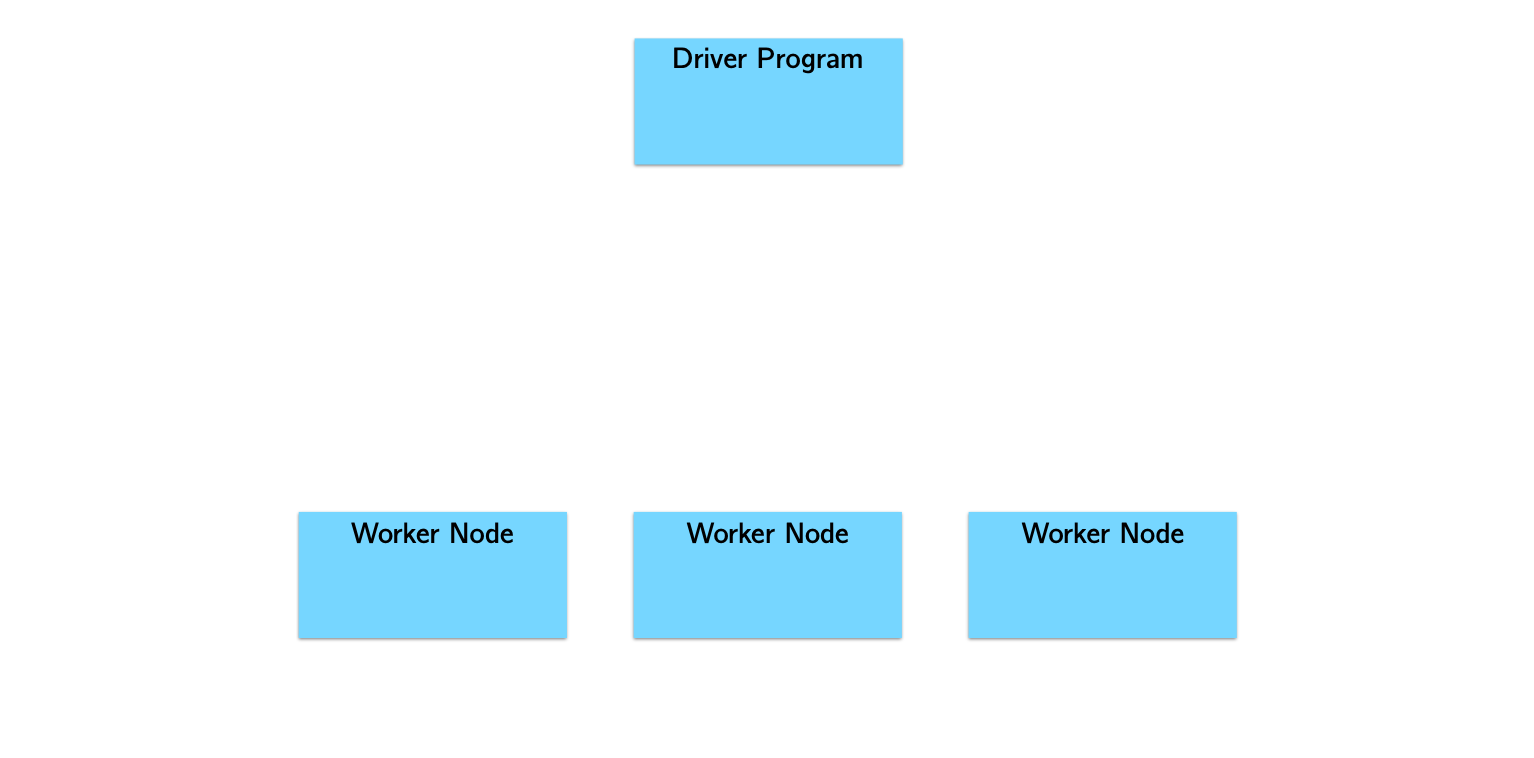
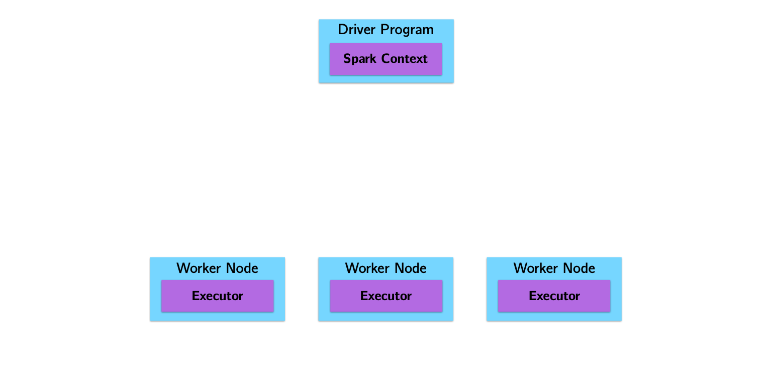
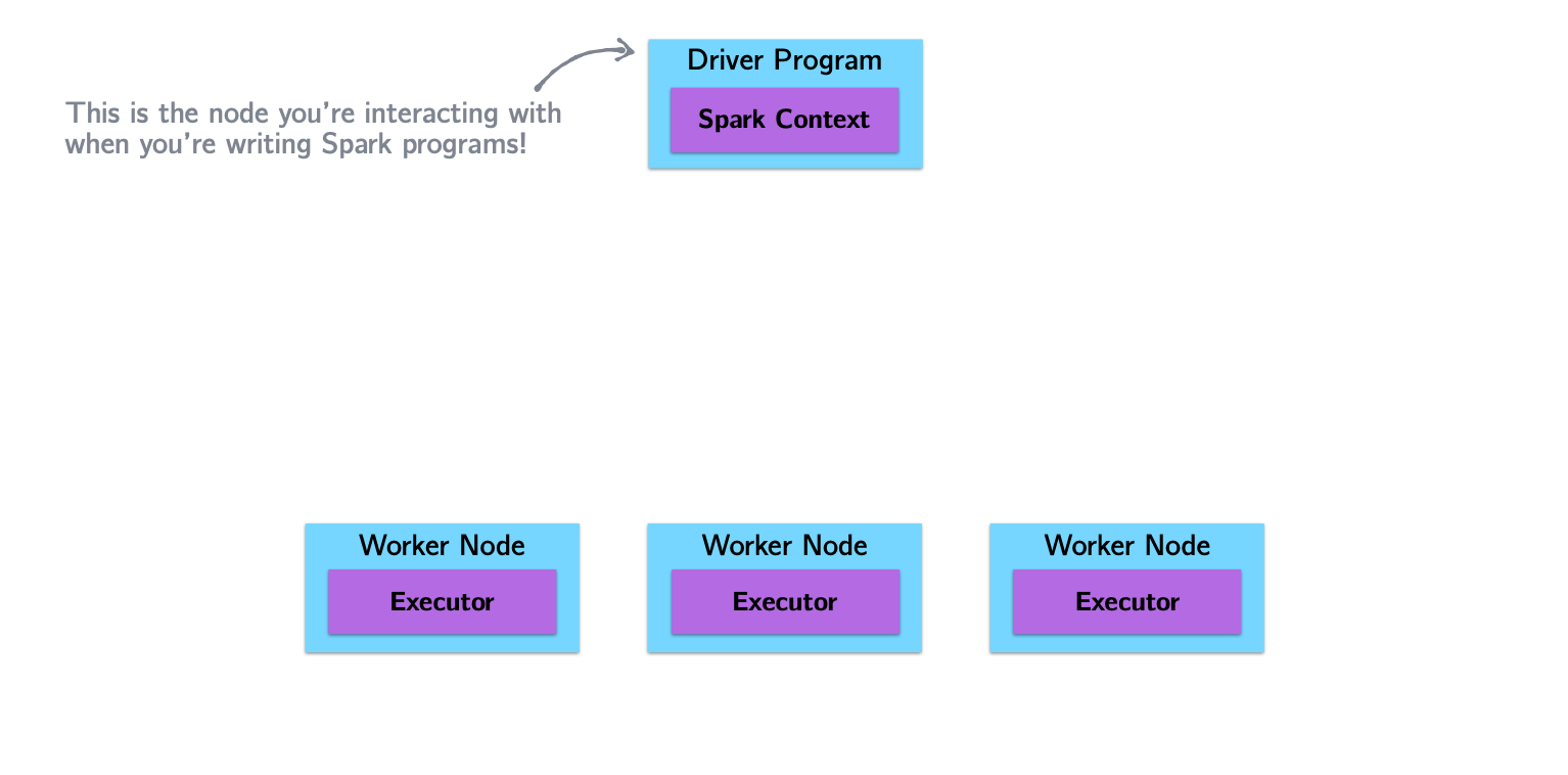
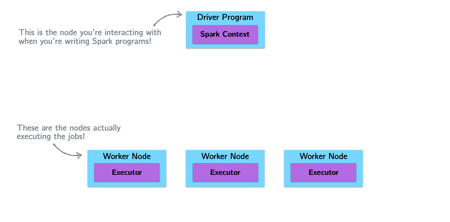
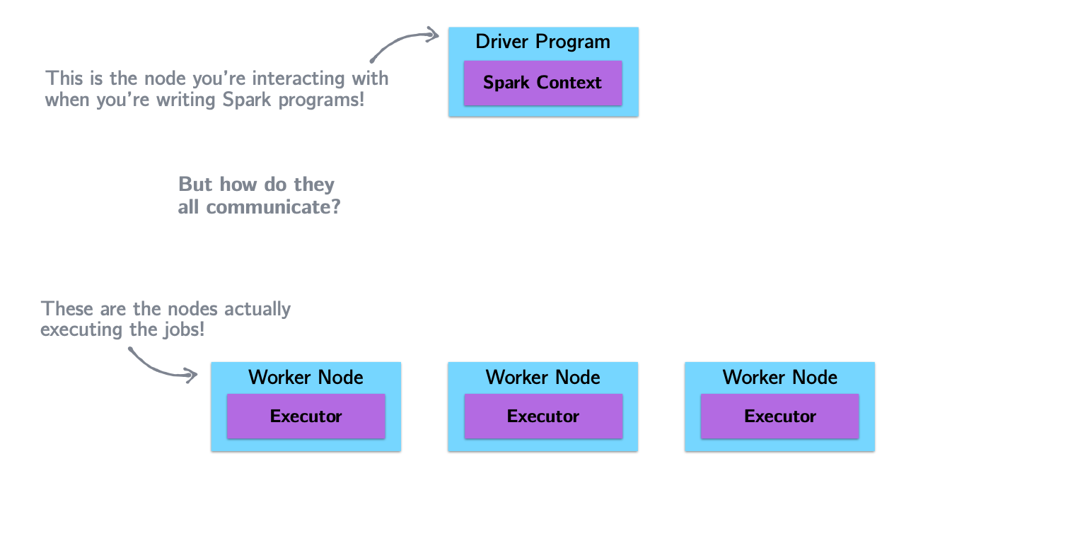
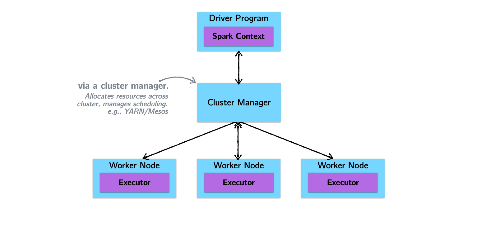
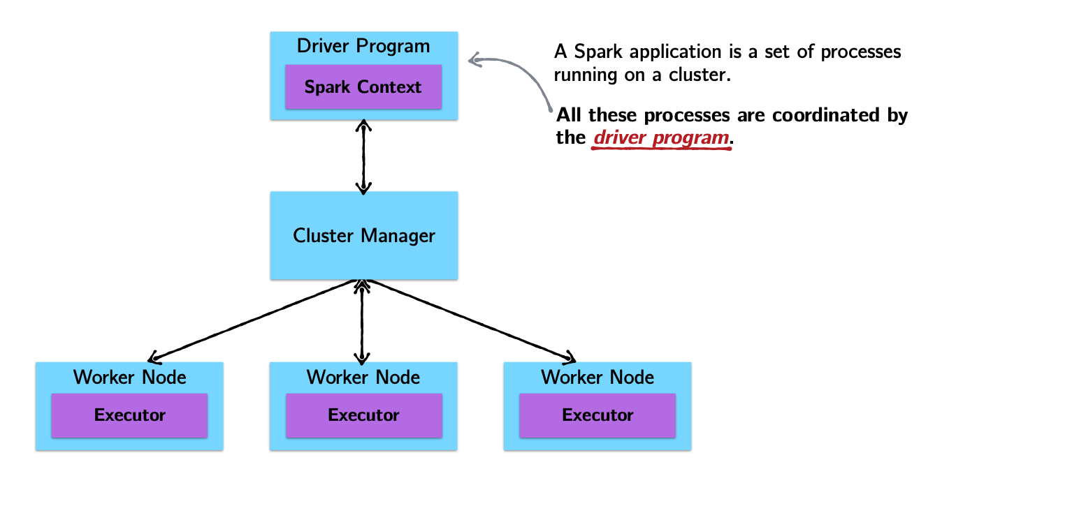
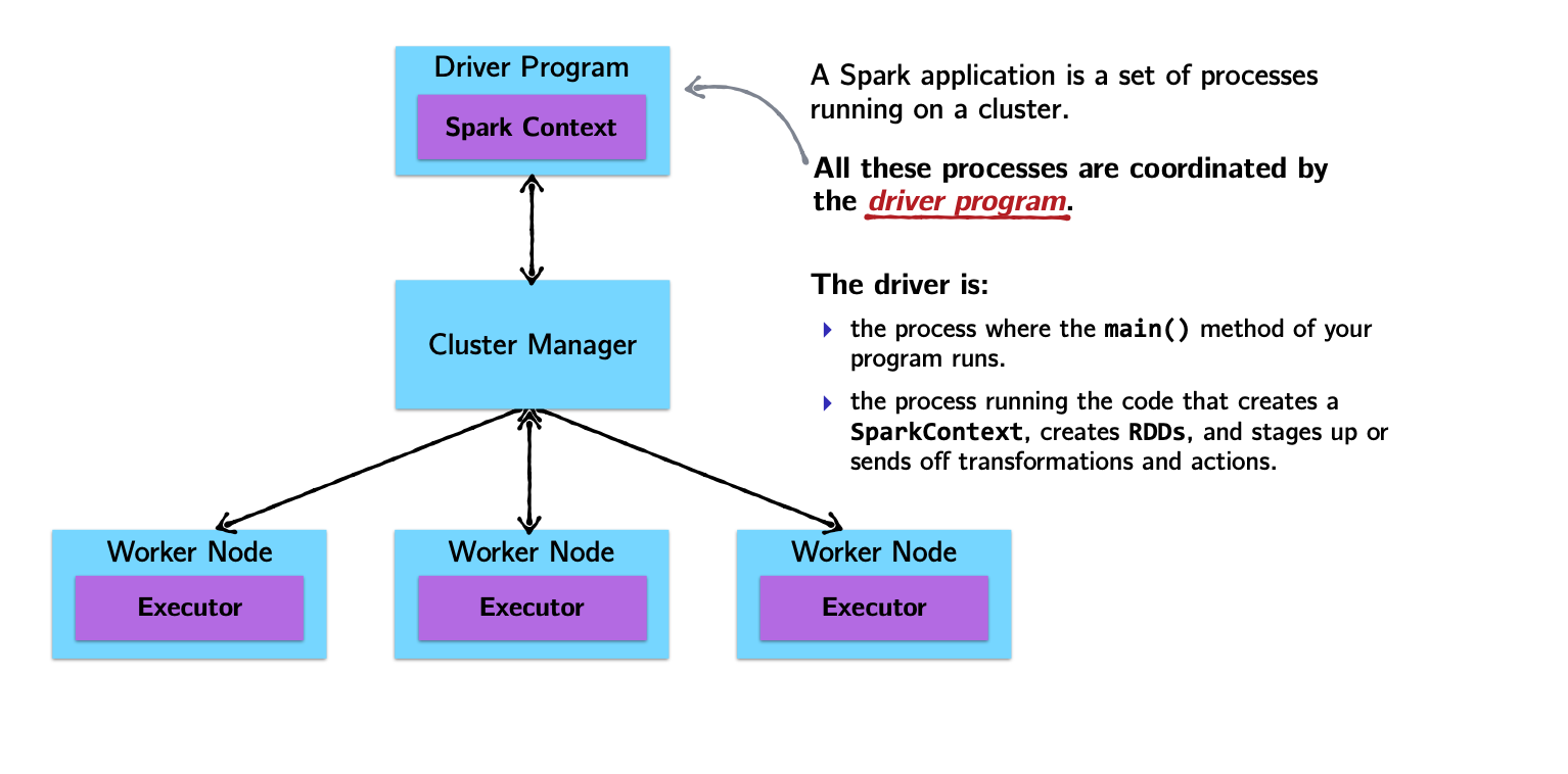
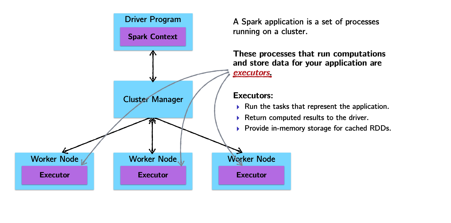
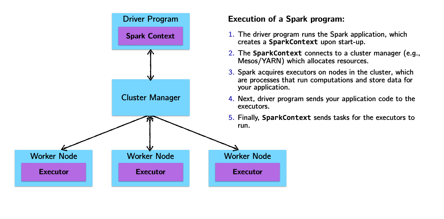
Spark Architecture and Job Flow
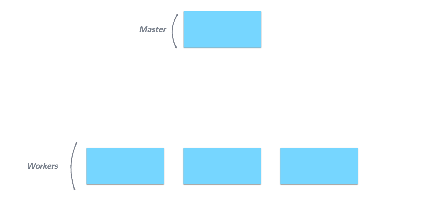
Spark vs. Hadoop
| Hadoop Limitation | Spark Approach |
|---|---|
| For iterative processes and interactive use, Hadoop’s mandatory dumping of output to disk is a huge bottleneck. In ML, users rely on iterative processes to train-test-retrain. | Spark uses an in-memory processing paradigm, lowering disk IO substantially. Spark uses DAGs to store transformation details and does not process them until required (lazy). |
| Traditional Hadoop applications needed data first copied to HDFS and then processed. | Spark works equally well with HDFS or any POSIX-style filesystem. |
| Resilience required a data-localization phase writing to local filesystem. | Resilience in Spark is achieved by DAGs — a missing RDD is re-calculated by following the path from which it was created. |
| Hadoop is built on Java; non-Java scripts require Hadoop Streaming. | Spark is developed in Scala with a unified API: use Spark with Scala, Java, R, or Python. |
Introducing the RDD
Example: word count (yes, again!)
The “Hello, World!” of programming with large-scale data.
That’s it!
Transformations and Actions (key Spark concept)
![]()
How to create an RDD?
RDDs can be created in two ways:
Transforming an existing RDD: just like a call to
mapon a list returns a new list, many higher-order functions defined on RDDs return a new RDDFrom a
SparkContextorSparkSessionobject: theSparkContextobject (renamedSparkSession) is your handle to the Spark cluster. It defines methods to create and populate a new RDD:parallelize:converts a local object into an RDDtextFile:reads a text file from your filesystem and returns an RDD of strings
Transformations and Actions
Spark defines transformations and actions on RDDs:
Transformations return new RDDs as results.
Actions compute a result based on an RDD, which is either returned or saved to an external filesystem.
Transformations and Actions
Spark defines transformations and actions on RDDs:
Transformations return new RDDs as results.
Transformations are lazy — their result RDD is not immediately computed.
Actions compute a result based on an RDD, which is either returned or saved to an external filesystem.
Actions are eager — their result is immediately computed.
Common RDD Transformations
| Method | Description |
|---|---|
map |
One-to-one transformation — transforms each element into one element of the result |
flatMap |
One-to-many transformation — transforms each element to 0 or more elements |
filter |
Returns an RDD of elements that pass a boolean filter condition |
distinct |
Returns RDD with duplicates removed |
Common RDD Actions
| Method | Description |
|---|---|
collect |
Returns all distributed elements of the RDD to the driver |
count |
Returns the number of elements in an RDD |
take |
Returns the first n elements of the RDD |
reduce |
Combines elements of the RDD using some function and returns the result |
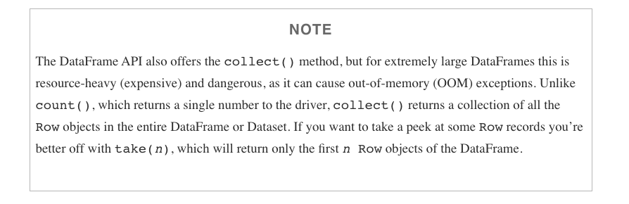
collect CAUTION
Another example
Let’s assume we have an RDD of strings containing gigabytes of logs from the previous year. Each element represents one log line.
Assuming dates come as YYYY-MM-DD:HH:MM:SS and errors are logged with prefix “error”…
How would you count errors logged in December 2019?
Spark computes RDDs the first time they are used in an action!
Caching and Persistence
By default, RDDs are recomputed every time you run an action on them. This can be expensive if you need to use a dataset more than once.
Spark allows you to control what is cached in memory.
To tell Spark to cache an object in memory, use persist() or cache():
cache()— shortcut for default storage level (memory only)persist()— customizable to memory and/or disk
Using memory is great for iterative workloads
DataFrames
DataFrames in a nutshell
DataFrames are…
Datasets organized into named columns
Conceptually equivalent to a table in a relational database or a data frame in R/Python, but with richer optimizations under the hood.
A relational API over Spark’s RDDs
Because sometimes it’s more convenient to use declarative relational APIs than functional APIs:
selectwherelimit
orderBygroupByjoin
Able to be automatically aggressively optimized
SparkSQL applies decades of research on relational optimizations in the database community to Spark.
DataFrame Data Types
SparkSQL’s DataFrames operate on a restricted (yet broad) set of data types. Most common:
- Integer types (at different lengths):
ByteType,ShortType,IntegerType,LongType - Decimal types:
FloatType,DoubleType BooleanTypeStringType- Date/Time:
TimestampType,DateType
A DataFrame
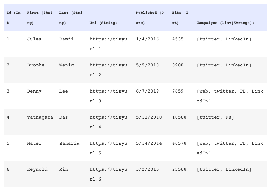
Getting a look at your data
There are a few ways to inspect DataFrames:
show()— pretty-prints theDataFramein tabular form; shows first 20 rowsprintSchema()— prints the schema of yourDataFramein a tree format
Common DataFrame Transformations
Like RDDs, transformations on DataFrames:
- Return another
DataFrameas a result - Are lazily evaluated
Some common transformations include:
| Method | Description |
|---|---|
select |
Selects a set of named columns and returns a new DataFrame |
agg |
Performs aggregations on a series of columns |
groupBy |
Groups the DataFrame by specified columns, usually before aggregation |
join |
Inner join with another DataFrame |
Other transformations include: filter, limit, orderBy, where.
Specifying columns
Most methods take a Column or String, always referring to some attribute/column in the DataFrame.
You can select and work with columns in three ways:
Using $ notation:
df.filter($"age" > 18)Referring to the DataFrame:
df.filter(df("age") > 18)Using SQL query string:
df.filter("age > 18")
Filtering in SparkSQL
The DataFrame API provides two equivalent methods for filtering: filter and where.
is equivalent to
Use either DataFrame API or SparkSQL
The DataFrame API and SparkSQL syntax can be used interchangeably!
Example: Return the first and last name of all employees over 25 in Washington D.C.
DataFrame API
SparkSQL
Grouping and aggregating on DataFrames
Common tasks on structured data:
- Grouping by a certain attribute
- Doing some kind of aggregation on the grouping, like a count
SparkSQL’s groupBy returns a RelationalGroupedDataset with aggregation functions: count, sum, max, min, and avg.
How to group
- Call
groupByon a specific column - Followed by a call to
agg
Actions on DataFrames
Like RDDs, DataFrames have their own set of actions:
| Method | Description |
|---|---|
collect |
Returns an array containing all rows to the driver |
count |
Returns the number of rows |
first |
Returns the first row |
show |
Displays the top 20 rows |
take |
Returns the first n rows |
collect CAUTION
Limitations on DataFrame
- Can only use DataFrame data types
- If your unstructured data cannot be reformulated to adhere to a schema, it would be better to use RDDs.
Modern Spark: Performance Improvements
Spark 3.x: Adaptive Query Execution (AQE)
AQE re-optimizes the query plan at runtime based on statistics collected during execution — something the static planner cannot do.
Enabled by default since Spark 3.2:
Three key optimizations:
Dynamic coalescing of shuffle partitions — merges small partitions after a shuffle to reduce overhead
Converting sort-merge joins to broadcast joins — when one side turns out to be small enough to broadcast at runtime
Skew join optimization — automatically splits skewed partitions to balance the workload
AQE in action
Tip
AQE is most impactful for queries involving joins, aggregations, and shuffles — exactly the patterns common in ETL and analytics workloads.
Without AQE, Spark uses static estimates from table statistics (often stale or missing). With AQE:
- Fewer tasks → less scheduling overhead
- Better memory utilization → fewer OOM errors
- Faster joins → no manual broadcast hints needed
You get this for free in Spark 3.2+.